# A tibble: 5 × 8
  species island bill_length_mm bill_depth_mm flipper_length_… body_mass_g sex
  <fct>   <fct>           <dbl>         <dbl>            <int>       <int> <fct>
1 Adelie  Torge…           39.1          18.7              181        3750 male
2 Adelie  Torge…           39.5          17.4              186        3800 fema…
3 Adelie  Torge…           40.3          18                195        3250 fema…
4 Adelie  Torge…           NA            NA                 NA          NA <NA>
5 Adelie  Torge…           36.7          19.3              193        3450 fema…
# … with 1 more variable: year <int>
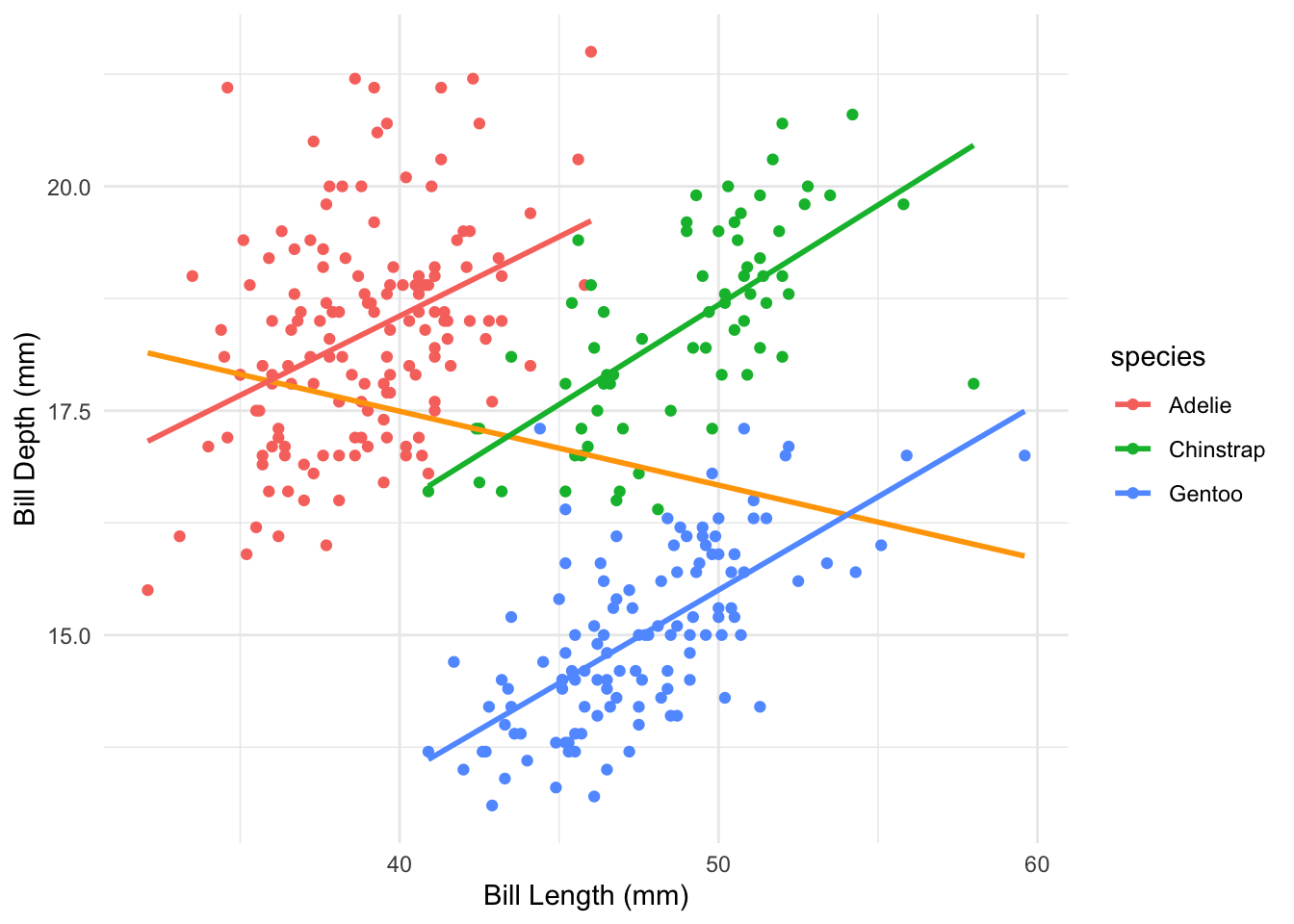
We have a few variables of interest which we can hypothesise may be interacting with each other. Let’s visualise the data:
Show the code
penguins%>%na.omit()%>%ggplot(aes(bill_length_mm,bill_depth_mm))+geom_point(aes(color =species))+geom_smooth(method =lm, color ="orange", formula ='y~x',se=FALSE)+geom_smooth(method =lm, aes(color =species), formula ='y~x', se=FALSE)+labs(y="Bill Depth (mm)", x="Bill Length (mm)")+theme_minimal()
The general linear model doesn’t seem too bad, but it doesn’t take into account potential interactions between species and the variables above. Conventionally we would test this by comparing two models, one which accounts for the interaction and one that doesn’t:
Show the code
model1<-lm(bill_length_mm~bill_depth_mm*species, data =penguins%>%na.omit())# summary(model1)model2<-lm(bill_length_mm~bill_depth_mm+species, data =penguins%>%na.omit())# summary(model2)anova(model1, model2)%>%tidy()
# A tibble: 2 × 6
  res.df   rss    df sumsq statistic    p.value
   <dbl> <dbl> <dbl> <dbl>     <dbl>      <dbl>
1    327 1954.    NA   NA       NA   NA
2    329 2095.    -2 -141.      11.8  0.0000117
We see that the p-value is statistically significant, so we choose the model with the interaction term.
2.1 The tidymodels framework
2.1.1 Create the data splits and feature engineering recipes
Let’s now take the tidymodels approach to the same problem. We start by defining our data budget and splits:
Next, we will define the respective pre-processing recipes, one with the interaction term and another without it:
Show the code
# model without interaction:rec_normal<-recipe(bill_length_mm~bill_depth_mm+species, data=penguin_train)%>%step_center(all_numeric_predictors())# the model with interaction:rec_interaction<-rec_normal%>%step_interact(~bill_depth_mm:species)
2.1.2 Create the workflows
Now that we have our recipes we can proceed to create our respective workflows:
Show the code
# Define the modelpenguin_model<-linear_reg()%>%set_engine("lm")%>%set_mode("regression")# Workflows# normal workflow:penguin_wf<-workflow()%>%add_model(penguin_model)%>%add_recipe(rec_normal)# interaction workflowpenguin_wf_interaction<-penguin_wf%>%update_recipe(rec_interaction)
Let’s now fit our model to the data:
Show the code
## Fitting# use the last_fit() to make sure data is trained on # training dataset and evaluated on test dataset. penguin_normal_lf<-last_fit(penguin_wf, split =penguin_split)
Warning: package 'rlang' was built under R version 4.1.2
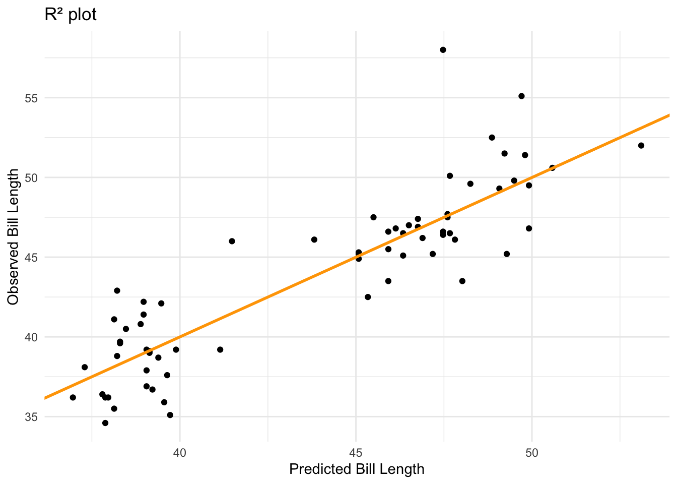
# plot model predictions:penguin_inter_lf%>%collect_predictions()%>%ggplot(aes(.pred, bill_length_mm))+geom_point()+geom_abline(intercept =0, slope =1, color ="orange", size =1)+labs(x ="Predicted Bill Length", y ="Observed Bill Length", title ="R² plot")+theme_minimal()
That’s it! We have successfully incorporated the tidymodels framework into the analysis ensuring robustness and sticking to good data practices.
Source Code
---title: "ANOVA with Tidymodels"title-block-banner: trueformat: html: code-fold: true code-summary: "Show the code" code-tools: true toc: true number-sections: true highlight-style: githublink-citations: trueimage: "penguins.jpg"---```{r, echo=FALSE, message=FALSE}pacman::p_load(tidyverse,tidymodels,palmerpenguins)```# The conventional approachUsually when conducting an analysis of variance we follow the steps outlined below:Step 1. Make model with multiple predictors no interaction.Step 2. Make another model with the supposed interaction.Step 3. `anova(model1,model2)`, if the p-value is significant, the more complex model is the one that you should select.# The tidymodels approachLet's take a look at the `Palmer Penguins` dataset:```{r}penguins %>%head(5)```We have a few variables of interest which we can hypothesise may be interacting with each other. Let's visualise the data:```{r}penguins %>%na.omit() %>%ggplot(aes(bill_length_mm,bill_depth_mm))+geom_point(aes(color = species)) +geom_smooth(method = lm, color ="orange",formula ='y~x',se=FALSE) +geom_smooth(method = lm, aes(color = species),formula ='y~x',se=FALSE) +labs(y="Bill Depth (mm)",x="Bill Length (mm)")+theme_minimal()```The general linear model doesn't seem too bad, but it doesn't take into account potential interactions between species and the variables above. Conventionally we would test this by comparing two models, one which accounts for the interaction and one that doesn't:```{r}model1 <-lm(bill_length_mm ~ bill_depth_mm * species, data = penguins %>%na.omit())# summary(model1)model2 <-lm(bill_length_mm ~ bill_depth_mm + species, data = penguins %>%na.omit())# summary(model2)anova(model1, model2) %>%tidy() ```We see that the p-value is statistically significant, so we choose the model with the interaction term.## The `tidymodels` framework### Create the data splits and feature engineering recipesLet's now take the tidymodels approach to the same problem. We start by defining our data budget and splits:```{r}set.seed(1234)penguin_split <-initial_split(penguins %>%na.omit(), strata = species, prop =0.8)penguin_train <-training(penguin_split)penguin_test <-testing(penguin_split)```Next, we will define the respective pre-processing recipes, one with the interaction term and another without it:```{r}# model without interaction:rec_normal <-recipe(bill_length_mm ~ bill_depth_mm + species,data=penguin_train) %>%step_center(all_numeric_predictors())# the model with interaction:rec_interaction <- rec_normal %>%step_interact(~ bill_depth_mm:species)```### Create the workflowsNow that we have our recipes we can proceed to create our respective workflows:```{r}# Define the modelpenguin_model <-linear_reg() %>%set_engine("lm") %>%set_mode("regression")# Workflows# normal workflow:penguin_wf <-workflow() %>%add_model(penguin_model) %>%add_recipe(rec_normal)# interaction workflowpenguin_wf_interaction <- penguin_wf %>%update_recipe(rec_interaction)```Let's now fit our model to the data:```{r}## Fitting# use the last_fit() to make sure data is trained on # training dataset and evaluated on test dataset. penguin_normal_lf <-last_fit(penguin_wf,split = penguin_split)penguin_inter_lf <-last_fit(penguin_wf_interaction,split = penguin_split)```### The ANOVA partBefore we compare the models using the `anova()` function, we have to extract the fitted models from the respective workflows:```{r}normalmodel <- penguin_normal_lf %>%extract_fit_engine()intermodel <- penguin_inter_lf %>%extract_fit_engine()anova(normalmodel,intermodel) %>%tidy()```We can get the model metrics using the `yardstick` package:```{r}penguin_inter_lf %>%collect_metrics()```Let's take a deeper look at the interaction terms:```{r}intermodel %>%tidy()```Finally it may be useful to plot the results:```{r}# plot model predictions:penguin_inter_lf %>%collect_predictions() %>%ggplot(aes(.pred, bill_length_mm)) +geom_point() +geom_abline(intercept =0, slope =1, color ="orange", size =1) +labs(x ="Predicted Bill Length",y ="Observed Bill Length",title ="R² plot") +theme_minimal()```That's it! We have successfully incorporated the tidymodels framework into the analysis ensuring robustness and sticking to good data practices.